Saturday, April 1, 2017

A 7-Year 10-Meter Es Propagation Study Using PropNET - Part 1 of 5

Please credit PropNET.org and Art Jackson KA5DWI if it used outside this Blog. Thanks
Releasing this Study after a 6 Year Delay:
This was the final study after 7 consecutive years of observing, recording, and analyzing 10-Meter PropNET data for the Spring/Summer Es season. I had published my 5-Year Study for the Proceedings of the Central States VHF Society Conference in 2010, updated for a 6th year and published it and presented it to the conference in 2011.

In 2011, Solar Cycle 24 had finally began its rise and in early May 2012 a hot-water line broke under the slab of the Shack and resulted a 45 day downtime as repairs were completed.  During 2012, the teaching profession took all of my time, but was able to finish two drafts of a 7-Year analysis. Early 2013 was the beginning of another rough year personally. My wife and I decided that retirement was in our immediate future. I looked to publishing the 7-Year Study again, but after reviewing 2012 and 2013 data, it was obvious that the past 2 seasonal results were contradictory to the past Study. Solar Cycle 24 had a strong negative effect on Es and this study was irrelevant.

In the Spring of 2014, I retired and moved to the high desert of Arizona.  In January 2016, I released on the Blog what Solar Cycle 24 had done to Es propagation. I did not participate in PropNET, but saw indications that Es propagation had returned to some extent using Weak Signal Propagation Reporter (WSPR).

I believe that this study is now relevant. We are quickly approaching the bottom of Solar Cycle 24 and a return to the properties seen in the Study will now return.

Interests and Curiosity:

I believe that I came from the last generation of Citizen Band Radio operators who took the operating skills learned there and used them to operate proficiently in Amateur Radio.  Although I agree that the old “good buddy” days changed the Citizen Band for the worse, it helped a large number of those operators to become good Hams.  The early CB operators, whether they wanted to or not had to learn to operate in and around occasions when the ionosphere lit up and was reflecting signals.  Good ground wave contacts were virtually impossible at times.  Many would operate very late at night for local rag-chews because it was the only time that the 11-Meter band was quiet.  It was not uncommon at these late hours to complete (accidentally although illegal) a contact with someone 500-1000 miles away.  The term “short-skip” was used to describe this condition that what today is called Sporadic Es propagation.    

Since becoming a Ham in early 1979, the 10-Meter Ham band has always been one of my favorite places to operate. I was lucky that during this time, 10-Meters was roaring with DX as Cycle 21 was nearing its peak.  The band was pure DX.  As a Novice, I remember listening for European beacons at the upper end of the Novice portion (CW from 28.100 - 28.200 MHz) and then moving back to the low end and working many of them till about noon local time. In the late afternoon, 10-Meters was full of both Asian and Oceania signals. During the fall and winter months the band was quite predictable. Using George Jacob’s - W3ASK “Shortwave Propagation Handbook”, his monthly article in CQ Magazine, plus the latest WWV solar indices it was not too hard to figure out when and to where 10-Meters was open.

I collected a large number of countries with relatively low-power, a good 10-Meter Yagi (a CB conversion), and a good curiosity and understanding of F2 propagation. Except for some occasional Central and South American signals, once it was 2 to 3 weeks after the Spring Equinox, 10-Meters flatly died out.  That sudden loss of propagation resulted in many to run off to other bands and overlook the development of Es propagation later in the month of April and early May.  

I was a FM/TV Broadcast Band DX’er well before becoming a Ham, and afterwards once I became a Ham. My first year as a Ham, I realized as DX activity on the lower television channels was occurring, 10-Meters was also open to regions not normally open in times of F2 propagation.  I suddenly remembered my past CB experiences of what we called “short-skip”.  Actually too late into the Es season, I enjoyed a few good Es QSOs in the CW portion of 10-Meters before the F2 propagation finally showed up again in September.

My interest in “Mode A” Satellites (2-Meters up/10-Meters down) in the early 1980’s resulted in also becoming active in 2-Meter SSB, known as Weak-Signal.  I clearly remember hearing N. American 10-Meter FM repeaters and operators in between AO-10, RS-5, 6, 7 and 8 and then working several more SSB and CW QSOs on 10-Meters during the Spring and Summer. The end result of my satellite activity was my first 2-Meter SSB Es QSO. I have found nothing more exciting than working 2-Meter Es and my curiosity about this Es grew.

Throughout the years on 2-Meter SSB, I have operated with an extremely modest station.  I have always attempted to be ready and waiting on any propagation opportunity rather than creating my own by putting together a “Big Gun” set-up.  I have achieved a great amount of success on 2-Meter SSB with that effort (43 states, 202 Grid Squares) thanks in part to being prepared for many Es openings.  In the 1980’s I learned that listening to 10-Meters, along with watching for signals on analog TV Channels 2-7 was the perfect way to be ready.  On a couple of occasions, I have worked the same station on 10 and 2-Meters within the same Es opening.  In May 1986, I worked my 50th 10-Meter state (Oklahoma) on 10-Meter Sporadic Es just as 2-Meters opened up.  I completed a 1450-mile QSO on 2-Meters in that same opening.  I always noticed that some of the best 2-Meter Es openings I had experienced were preceded, during or followed by excellent 10-Meter Es events.

In 1987, I became active on 6-Meters, and the following year on AMSAT-Oscar 13 Modes B and J.  Sadly my 10-Meter activity suffered in the process. Still it was not uncommon that at least during Field Days that I would operate “1C” (mobile) running on 10-Meters searching for that potential Es opening. Due to work and travel, from the mid 1990’s until after 2000, my Ham activity was again very limited.  I still tried to make an effort to at least make sure the rigs worked, and would show up on 10 and 6-Meters during Field Day and other summer contests to experience Es propagation.  My curiosity never waned. On numerous occasions I would discuss and share experiences with others as to what was behind Es propagation. I spent many an afternoon and evening rag-chewing with other VHF aficionados about the phenomena.  I also seemed to be more thrilled making 10, 6 and 2-Meter Es QSOs than most of the F2 ones on the HF bands.

In 2001, I retired from a 30-year profession and again had an opportunity to operate what was my favorite HF band.  Ham Radio had changed much in a few short years, and I was somewhat surprised by the lack of activity on 10-Meters.  I found the band much too quiet during the spring and summer months. I also personally concentrated on 6-Meters as we were enjoying the peak of Cycle 23.  In 2002 as my Ham activity was on the upswing, I ran across a new Ham Radio activity called Beaconet on a VHF/UHF digital interest Yahoo Group. The Beaconet group was using the BPSK31 mode instead of AX.25 Packet for identification.  I was impressed with BPSK31 because of its ease of use between a rig and the computer sound card without utilizing a TNC.  I had completed a few BPSK31 QSOs on HF and learned that many signals could be copied and worked in a narrow bandwidth and minimal conditions.   

In 2003, I could not locate the Beaconet group.  I inquired on the Yahoo Group that I first noticed Beaconet and got an immediate response from Ev Tupis, W2EV.  Beaconet was alive and well, but it was now called PropNET.  Immediately, I was drawn towards doing something positive with it.  In late spring of 2004 while using software named MultiPSK, I participated more in a “lurker” (listening only) mode on 10-Meters.  I was very satisfied with the results. Using a sequenced formatted transmission, each reception of a PropNET participant’s signal was logged by the software and a daily “Catch Report” was generated.  Many of my past memories of how and when Es formed were being jogged about, and a number of old theories were being recalled.  I could now capture, then use from a statistically sound sampling of real data that I could compile, review, and analyze. I decided that for the 2005 Spring/Summer Es season I would become a full-time participant in PropNET in order to produce a propagation study.

For 2005, W2EV Ev Tupis, N7YG Jeff Stienkamp, and KF6XA Dave Donnelly had made major changes for the betterment of the entire PropNET group. It brought in more participants and raised the sample of users to make a better study.  New software called PropNetPSK easily configured your own transmissions, logged complete and partial receptions of PropNET transmissions, produced an hourly Catch Report, and most important now updated real-time propagation maps via a Telnet connection known as LiveXchange (LiveX). With the ability to see your call on a map, interest picked up in the Ham community. I had a sampling that would easily satisfy the “Central Limit Theorem” used in statistical workings. In late April 2005 I became a full-time participant of PropNET.

Despite quite a few years of working Es, many of my personal opinions and theories immediately proved to need refinement.  I compiled a statistical summary of the 2005 Spring/Summer Es season and my first thought was that I needed to it again for 2006. The data for 2005 was clean, but it needed more support.  In 2006, overall conditions seemed to be much better.  The data gathered was much improved, although at times I had more problems with the software. After gathering these 2 years of data, many of trends that occur with Es were more clearly defined, but still a third year of data was needed to insure that the prior two years were consistent.

I did my absolute best on the third year to remove any of the past difficulties I had within the prior two. The goal was to produce reliable and clean data. The third year was the best and most thorough year of all. With this third year I compiled a comprehensive 3-year study for those years of data.  Unfortunately, working on a Bachelor’s Degree and starting a teaching career delayed its completion late enough that I decided to participate for a 4th year to put the “icing on the cake”.  It was a good decision.  Once again the teaching career, my certification and a well desired vacation during the best time to present a study put me in the position to add a 5th year.  By the 4th year, consistent trend-lines had developed,in and the 5th, 6th and the 7th year’s data made them more precise and trend lines that were closely tied to actual data.

The fifth year (2009) was the minimum of solar cycle 23. Conditions were excellent and results had a positive effect on my analysis. The PropNET group decided during the fall of 2009 to change its 10-Meter operating frequency from 28.131 to 28.1188 MHz.  The move placed PropNET activity 1200 Hz below the recognized 10-Meter PSK31 calling frequency and allowed the software to capture non-PropNET activty.  I did have concerns that it would affect the data gathering efforts, but once the season was over it actually complimented it.  With the arrival of Cycle 24, the “beginning to end” of season trends were harder to define.

In 2011, the ability of PropNET participants to “robot” was added to the software.  In addition, if the 1500 Hz area was covered by a signal, the PropNET package was transmitting below or above 1500Hz.  I was not convinced that this improved capture numbers, nor did I participate as a “Robot” as it was counterproductive to my intents, hearing PSK31 signals.

No one year was perfect, but any inconsistencies never had a serious affect on the overall numbers gathered. All attempts to be consistent in operations were maintained throughout the 7 years as to working habits, rigs and antennas.  The same software PropNetPSK (PNP) was used on three very similar desktop computers; except that one ran Windows ME, one ran Windows XP Home and the third ran XP Pro. 

Operating and Background Information:

Location (QTH): North Richland Hills, Texas (Northeast Tarrant County near Ft. Worth). Grid Square – EM12ju.  Terrain: 640 feet Elevation and hills 50-60 feet higher one-third to one-half mile northeast to east.

Rig Transceiver – Yaesu FT-747GX 
Auto ID transmissions were set normally at 5 to 6 times per hour. The BPSK31 Auto ID lasts for about 30 seconds (2.5-3 minutes an hour). 57 minutes+ per hour are spent listening for other PropNET and Non-PropNET stations. 
It was operated in this mode normally from 07:00 to 23:00 local Central Daylight Time (-5 hours UTC) for the first 3 years and 24 hours for the last 4.

Rig Lurker (monitor only) – Radio Shack HTX-10.
This rig was an outstanding performer for a receive-only operation. It was run during late night and early morning hours for 3 years.  I also ran this mode while on any trip or vacation. Its good sensitivity and AGC was perfect for the reception of BPSK31 signals and outperformed the Yaesu for non-PropNET signals as it is broad-banded (3,000 Hz).

Antennas: Primary antenna was a 3-Element Yagi (30+ year old Hustler converted CB) at 30 feet high and usually pointed east-north-east (70 degrees azimuth). The secondary antennas were a 120-foot Inverted-V Doublet, a Cushcraft ATV-3 vertical, a Lakeview 10-Meter Hamstick, or a 102 inch CB mobile whip used when weather conditions were a concern, or when I was on a trip for a few days.  At least three-quarters of my operating was with the Yaesu FT-747GX into the Yagi.

Computers: Dell Dimension P3 1 GHz WinME, P4 1.8 GHz WinXP Home, and P4 3 GHz WinXP Pro desktop computers.

Software: Versions 2.X.X.X, 3.X.X.X and 4.X.X.X PropNetPSK (now PNP) developed and maintained by N7YG Jeff Steinkamp

PropNET and PropNETPSK Program Operations:

  1. The software is configured for the band operated, listening bandwidth, IMD channels, AFC parameters, and other miscellaneous program settings.
  2. A “PHG Code” (used in APRS) for power output, antenna gain, auto-ids per hour, antenna height above terrain, height above sea level, and antenna direction is configured.
  3. An example of the PropNET Auto-ID
    “For Information, please visit http://www.propnet.org
    ka5dwi>hy:[em12ju]PHG715205/^FC56”
    Call, Band (“hy” for 10-Meters), Grid Square, PHG code as configured, and 4 characters that validates the configured string.
  4. The PropNetPSK software, via the sound card captures and logs the data string. If complete and correct, it is logged by call, grid square and designated as a “Capture”.  If identified as a data string, but it is incomplete or not read correctly, it is designated as a “Partial/Fragment”.
  5. From the receiving station’s Internet connection, both Captures and Partial/Fragments were sent via LiveX to a Website (first years FindU, now direct to PropNET) to update propagation details and real-time maps. Data can now be extracted into a CSV file for report building.
  6. For five years a “Catch Report” was generated at 23:59:59.  The daily report was often sent to a Yahoo Group for archival. For 2 years all data sent via LiveX has been archived and extracted into a CSV data file for data collection.


    A 07/16/2009 10-Meter 24 hour map generated at PropNET.org from LiveX data.
Former Catch Report Excerpt Generated by PropNetPSK:

KA5DWI PropNET^31 - HY 06/29/2007 23:59:58 Z
                                   | Catches per UTC hour |
Call     Grid    Azm   Dist First 000000000011111111112222 Last  Config
          SQ           (KM) Heard 012345678901234567890123 Heard PHGVRA
-----------------------------------------------------------------------
WB8ILI  EN82PQ     49  1675 01:36  36          423       2 23:53  HY-PHG529765
WD4RBX  EM84NN     81  1338 13:14              341         15:05  HY-PHG500066
K4RKM   EM85VF     79  1405 14:52               21       3 23:50  HY-PHG703066
NZ9Z    EN64BD     32  1492 12:33             45461171   1 23:50  HY-PHG339556
K8VGL   EM69UT     51  1245 12:52             185 1      1 23:33  HY-PHG301066
KI0GU   EN35HF     13  1413 23:26                        2 23:26  HY-PHG7296A6
KC0EFC  EM28OX     17   714 23:29                        1 23:29  HY-PHG700066
KA5DWI  EM12JU      0     0 00:05 656         366666666666 23:54  HY-PHG315365
KD5LWU  DM57RI    295  1144 16:45                 13 1   3 23:17  HY-PHGA16069
N7YG    DM42NF    266  1282 16:15                 2A983772 23:15  HY-PHG513067

Partial Catch List:
23:53:39 HY - ÷e2uk8vgVnhy:[em69ut]PHG301066/^CF16 1753Hz
23:50:14 HY - k4rkm>hy:mqFvf]PHG7030io tr hTete1A8A* 1537Hz
23:46:51 HY - wbõe i>hADooe  2xu]Per10661/^962B 1551Hz
23:43:38 HY - k8vge  5 •[ m69ut]PH13a  66/^CF16 1750Hz
23:39:58 HY - k4rkm>hy:[eoÁheO5vf]PHG70306ítwh  e/^|A* 1533Hz
23:39:06 HY - i 'efc>hy:[em28ox]PHG700066/^BAE7 1541Hz
23:36:50 HY - wb4jfiehH-Eem92xu]PH3.sao aa t/^ie±iB 1554Hz
23:34:01 HY - lTpnanteel r t  rNyeÌt  rner    e   I t re 1402Hz
23:33:36 HY - k8vgl>hy:[em69ut]PHG301d66/t* 1755Hz
23:29:51 HY - n te.t wwwIPropNET  e .tos eai e  naekm>hy:[e5]PHG703066/^1A8A 1538Hz
23:23:36 HY - lem69ut]PHG301u66/^CF16 1754Hz
23:19:45 HY - k4rkm>hy:[em8"vfeHvd0p ee©oï1AÑ* 1534Hz
23:17:37 HY - kd5lwu>hy:[dm57ri]PHGA160O9/^83B8* 1431Hz
……………………………………………
Created with PropNetPSK © Version 2.1.0.2

Daily Report Extracted from LiveX data provided by the PropNet Website (replaced Catch Report):

Developed by Dave Donnelly, KF6XA

PropNET Participants:

The one statistically sound part that the PropNET Project provided was an excellent sample of participants.  At any one time, no fewer than 7 North American PropNET participants were active.  During the daytime and evening hours at least 20 were active.  Unfortunately, North America is not shaped like a circle. Although my QTH was located close to the middle of the United States, PropNET participants were not evenly distributed and using the same antennas, rigs and operating habits.  The end result was that the volume of these captures was skewed towards specific areas of the country. Due to consistently excellent propagation and a cluster of PropNET participants, one-half of the total captures occurred towards the east (67.5° to 112.5° azimuth) from my North Texas QTH.

Although skewed towards the east, propagation to that direction was generally the best indication for a slow or highly active day.  As the good conditions to the East started, for the rest of the day the other directions would follow. The population of active PropNET users results in good numbers from Southeast to North to West.  Due to my location and PropNET population, numbers were much lower to my South and Southwest.

As noted, most of the participating stations in the seven years were clearly located in the eastern half of the United States. The vast majority of those stations participating in the PropNET Project have been captured at one time or another by my operation.

The Data:
After 7 years of collecting PropNET captures and partials, the final results were as follows:

PropNET participants only:
Dates: April 25 to August 15, 2005-2011 Documented (Measurements taken from April 20 to August 31)
Captures and Identified Partials: 87,001 (Average 12,428 per season, 110 per day, near 5 per hour and 10 per active hour)
Active Hours with Propagation: 8,611 out of 18,984 possible hours (45.36% = 10.9 hours/day)
Calls: 198
Grid Squares: 123
States - 41, includes Hawaii and 2 Canadian Provinces
DX: Puerto Rico and Venezuela

The Arduous Task of Compiling the Data:

I came from a financial background (Financial Institution operations) and have been working with statistical and financial data for over 30 years. I have worked with many word processing, spreadsheet, database, and file extract/data import software packages since the creation of the modern personal computer.  Compiling this data was “second nature” to me. I could compile a season’s worth of statistical data within a few days.    

The data used in this analysis was primarily derived from the PropNetPSK “Catch Reports” and files extracted from LiveX created by KA5DWI.  On several occasions, due to the failure of the software or problems between LiveX and me, reporting was manually calculated. This procedure was highly accurate.

The capture data analysis only includes stations captured at the QTH of KA5DWI in grid-square EM12ju. It does not include stations that captured KA5DWI, nor any other PropNET participant station’s data.  I used nearby participants in the same time zone on rare occurrences (primarily power failures) for probability statistical data only due to any software or hardware failures at my QTH. 

Each daily “Catch Report” or data export was opened and then parsed into an Excel spreadsheet for each annual Es season.  Proper accounting procedures were used to insure that totals were correct and verified throughout the entire process. Prior to 2009, partial/fragment data was loaded into separate Excel worksheets and with the use of the “Data-Filter” routine, were identified and assigned as catches by call, date, and time.  These identified partials were added to the totals derived from the Catch Report detail.

The only inaccuracies that occurred in the compiling of data are due to multiple captures from another station’s single transmission.  Whenever signals were strong, it was not uncommon for the two or three channels (IMD) in the software to each capture the transmission. The software was not capable of eliminating duplicate entries. Strong BPSK31 signals that were over-modulated tended to do likewise. I was only able to remove duplicate partials. I am certain that in the best conditions, some totals were inflated. These were not large enough to have skewed the overall results, but we will consider them weighted since excellent propagation conditions were the cause.  Duplicate captures will have no bearing on probability statistics.  No major changes to software settings were made during the season that would affect or change the controlled conditions.  Therefore, inflated accumulated numbers occur evenly throughout each season.

Statistically the numbers compiled are sound.  There was at any time during the sevens years gathered enough active stations to produce a statistically reliable sample of data (Central Limit Theorem).  Of the 198 different stations captured, 18 were captured near or well above 1,000 times in 7 years.  The analyzed captures and identified partials averaged almost 12,500 per year.  34 PNP stations account for 90% of the total data.

The Spring/Summer “Es” Season:

When the first individual season study was first begun in 2005, my opinion based on experience was that for 10-Meters, the Spring/Summer Es season occurred from about May 1 till August 11.  Once I compiled the data for 2005, I determined that I was slightly incorrect.  The season begins a few days earlier and ends many more days later.  I extended the data gathering efforts from April 20 till August 15 for the study.  I should have extended the end date of each seasonal study much later (2 weeks at least), but other obligations, such as pursuing a college degree kept me from doing so efficiently for the first four years. I still was active many of those days and did retain my data. To make up for the lack of activity, I used data primarily from John Ainsworth, N5XYO in DM90 to complete 2 more weeks of probability analysis to help better define the end of the Es season.   

The Purpose of the Study and What it shows:

I do not pretend to have any solid answers to what causes Es. Many others, most notably Emil Peacock –W3EP, Jim Kennedy – K6MIO/KH6, Patrick Dyer – WA5IYX, J.A. Pierce – W1JFO, and Melvin Wilson – W1DEI/W2BOC have investigated and documented the phenomena.  Others continue to analyze it today. But after my own operating experience and documentation, I began to believe that most were concentrating on the answers to its creation and that maybe there was some bias towards the normality and predictability of what Es will display.  I never believed that “Sporadic” was a good term to call it.   

The purpose of the study was to show that Es was a very natural and predictable propagation phenomenon, and that there was nothing too magical about it. I researched this on a mathematical, not a scientific basis.  Finally, it was incorrect for it to be called “Sporadic”.  I believe that this study clearly accomplishes it.  Es propagation of this nature should have a totally different description for its occurrence.  Along the way I made some interesting observations that should create forums for future discussions. I believe that the intensity of Es can influenced from outside elements.  But, in no way should these outside elements have any influence on the central point of the study in that seasonal Es are predictable.

The study is broken down into the following parts:
  1. Numerical activity, such as statistics yearly, daily, weekly, and hourly during the season.
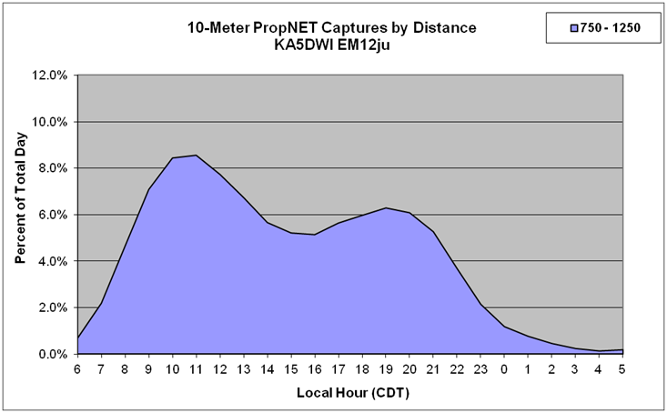
  2. Distance analysis hourly by segments.
  3. Directional analysis hourly throughout the season.
  4. Probability analysis by weekly segments, by week, by hourly segments, and hourly.
  5. Spring/Summer Es Seasonal Calendar.  

I want to thank everyone involved with the PropNET organization.  Without the founders, programmers, forward-thinkers, and its participants, a study of this magnitude could not have been accomplished.

Solar Conditions during this 7-Year Study:

I have experienced on many occasions solar conditions having both an adverse and positive effect on Es conditions. Most notably, I have observed enhanced Es thanks to the beginning of a minor magnetic storm from a coronal mass ejection (CME). Some of my best late season 2-Meter Es events were due to these events. On the other hand, many excellent Es events on 10 and 6 Meters were abruptly ended by solar flares.

The 7 years could not have been more perfect as we have experienced one of the most prolonged bottoms of a solar cycle. For the first 6 years, solar flux was never high enough to support F2 propagation. MUF never was higher than 21 MHz. The final year, 2011 was there any real indication of an F2 influence. The low levels of solar activity kept disturbances to a minimum, therefore having only a minor impact.  Only twice in 7 years could I determine a prolonged affect. The first was very early in the season of 2008 and the second in mid-July 2010.  In 2011, the sun had become much more active. Whether it had a negative affect on Es propagation is difficult to determine.  Although it was the 2nd lowest productive year, the least productive season was during the minimum of the cycle (2008).

The following charts show average solar flux and the Ap indices for the 7 year period and the spring/summer season:   
          
From 2005 to 2008, solar flux steadily declined.  In 2009 it increased slightly and by 2011 it had finally exceeded 2006 levels. The Ap indices declined in succession for five years.  Solar flux averaged 80 or below for 5 years, slightly above 90 and at 100 for one year each.

Disclaimer for the 7-Year Study

This 7-Year Study occurred at the end of Solar Cycle 23, the lull between, the beginning of Cycle 24. It ended as Cycle 24 began to take off. It was learned during Cycle 24, that the predictions of the beginning of the season, the peak of and the ending of the Spring/Summer Es season was much harder to define. Also, as Cycle 24 developed it had deterred Es activity. It was an exponential (mathematical) decline through the peak. See: http://ka5dwipropagation.blogspot.com/2016/01/how-solar-cycle-24-affected-10-meter.html
Now that we are entering the end of this solar cycle, this study should be relevant again.

Spring/Summer Es Intensity Year to Year:

Due to the ending of Cycle 23, I thought that we would see a consistent improvement each year until we reached the bottom of the cycle.  After 7 years I have noticed that although there are indeed year to year consistencies, Es have their own schedule.  If any pattern was recognized in the study, it was that there could be a 3 year cycle (2 good years, 1 not so good).

The individual year hourly percentage breakdown shows a clear dual-peaked diurnal pattern for the last 5 of the 7 years measured.  If the first 2 years are averaged, there is a dual peak.  Only 2 consecutive years were extremely close in their hourly patterns (2009 & 2010).

The preceding charts are running 3 consecutive years of actual hourly captures throughout the total 7 years measured.  As noted earlier in every three consecutive years, one year’s activity is typically less than the other two. 

Next: How he Season Begins and Ends

A 7-Year 10-Meter Es Propagation Study Using PropNET - Part 2 of 5

The Spring/Summer Es Season, From the Beginning to the End:

The chart represents the actual number of 10-Meter PropNET PSK31 captures at my location (North Central Texas) for each day from April 20 till August 15, 2005–2011.  At first it was difficult to see any clear trends using daily numbers, but within 5 years it finally called attention to several factors related to Es propagation. I was startled to see specific days being so active and other days close to those peaks were fairly quiet.  Each annual season measured in this study was 131 days (concentrated data on 113), in which nearly 20 days were extremely active. The other days measured show a steady increase once the season began, then a peak around the solstice, and slow decline into mid August.

To more clearly demonstrate trends and determine peaks, I used a daily averaging approach. It was begun in the first year of analysis (2005) in order to smooth out the daily trends and focus activity to specific dates of the season. The following chart shows the average number of daily captures 6 days prior to and including the day charted.  Rather than using actual dates, the chart indicates the number of days prior to and after the Summer Solstice (6/21).  The chart better displays concentrations of Es propagation.  The chart shows that from 22 to 12 days prior to solstice (5/31 to 6/09, 6/06 peak) was the most active period for Es.  In the latter years of the study, a peak developed just prior to the Summer Solstice. During the season there are 7 apparent concentrations of Es activity.

The events of a typical season show:
1. A quick rise in activity seven weeks prior to the summer solstice.
2. The absolute peak about 2 weeks prior to solstice.
3. A distinguishing lull approaching the solstice.
4. A second peak near the solstice.
5. A steady high rate of activity 2 weeks after solstice.
5. A gradual decline throughout the remainder of the season along with occasional bursts.

Rather than a perfect bell shaped curve, activity appears to be skewed to the right and is right-tailed. The median (midpoint) of the total captures in this study occurs on 6/22, the day after the Summer Solstice. The “median” capture point also proves that Es propagation is a seasonal phenomenon.


Trends appeared to be prevalent although captures varied greatly for day to day.  A polynomial regression analysis was applied to the 7 year daily average captures. Although not perfect, a good trend line was established at 2 degrees (x²). Raising the degree did little improvement to the coefficient of determination at .6432 (measured from 0 to1). This coefficient has improved year to year and each trend tightens.

The beginning of the season was on April 26. The peak of approximately 167 captures occurs on June 22.  The season trends towards an August 21 end. Trend line activity is at least 50% of peak from May 14 till August 2.  Activity is 90% of peak from June 4 to July 11.  Again, the trend line indicates rapidly early rise and late decline, with a skewing towards the latter half.

     
Another method to view Es activity was to chart the total PropNET captures it into one week segments.  The following chart shows total captures in one week periods from 8 weeks prior to and 8 weeks past the Summer Solstice. It is one of the only charts that show some inconsistencies in the season and leads to looking at outside influences to Es. In the first years, the 6th week of the season was the best. There was right skewing of the data during that time. In the later years of the study, the 8th through the 11th weeks rapidly caught up in total. The Summer Solstice occurs the 2nd day of Week 9.  A lull of total captures in weeks 7 and 9 was noticeable in the early years. It was not until 2008 (solar cycle bottom) that the 8th week became the most active of the season. One notable trend each year was an increase in activity beginning with Week 14 and Week 16.  For this reason, I should have extended the study at least two more weeks, 18 in total. It will be accounted for in the probability analysis.

The Time of the Day That Es Occur:

My belief from practical experience and with other researchers was that Es seemed to be best in the late afternoon/early evening hours.  I discovered in this analysis that it is the morning hours towards midday that are the best time for Es.  More operating activity from Hams generally occurs during the later hours of day, and that was the probable cause for the assumption.  The afternoon hours are still very active, but not to the level experienced in the morning hours. The afternoon hours still have unique characteristics.

All time charts are displayed in Daybreak (Sunrise) to Daybreak (Sunrise) order and expressed in Daylight Savings Time (Central).  At this location, the sun rose in the 6 AM (6) CDT hour and sets during the 8 PM (22) CDT hour.  10-Meter Es were decisively diurnal (daytime-patterned).  Therefore, it was best to display all results in daytime hours first, followed by evening and twilight hours.

The following chart is the number of Spring/Summer Es captures by hour for each year of the study. After seeing different Diurnal patterns between 2005 and 2006, this encouraged me to do a third year of participation to determine a true pattern.  The 2006, 2007 and 2008 data would look similar in many regards. The final 3 years (2009, 2010 & 2011) would display a more equal “dual-diurnal” pattern. What I got out of these charts was that each year does have similar trends, but each one has its own distinctive personality.

Once again to better display hourly trends, the next chart is displayed as a 3-hour average. For example, the plot for 6 AM is the average of 5, 6 and 7 AM.  Averaging does not change the overall totals, but smooths out the transitions between each hour.  This method works best in demonstrating what Es actually do.

After accumulating the 7 years together, it was very clear to see that Spring/Summer Es are diurnal and are generally better during in the late morning hours. Once the sun rises, Es rapidly increase. Once the sun sets, Es decline sharply.  Most dominant in 2007 through 2011, the overall chart shows a “dual-peak” diurnal pattern.

Activity Week to Week:

The following chart displays 3-hour average captures for the 16-Week Spring/Summer Es season (8 weeks each side of the Summer Solstice). The 6th week of the season is the most active and clearly appears similar in trends to the overall seasonal data chart. The 8th week grew rapidly the last half of the analysis and had a distinctive dual diurnal peak. The 1st, 2nd, and 13th weeks are least active, but clearly show a diurnal pattern as well. Only the early and latter weeks of the season fail to show a dual-peaked diurnal pattern.


Next: Distance Analysis

A 7-Year 10-Meter Es Propagation Study Using PropNET - Part 3 of 5

Distance Analysis:

One of the characteristics of Es that might be unknown is how propagation of the E layer changes during the course of a day.  I noticed into the second year of the study that many of the longer distance captures were occurring late into the afternoon. Using the distance calculation and data provided from the PropNetPSK software for each station captured, I was able to determine the average distance of the captures (in kilometers) for each hour of the day.

As I suspected, the longest distant PropNET captures do occur late in the afternoon during the 5 and 6 PM (17-18) local hours. Throughout the 7 years that data was collected, most of the longer distant captures would occur that occur in the morning.  The long distance captures to Hawaii, Puerto Rico, and the northeast and northwest corners of the United States would occur late in the afternoon. In the morning daytime hours as 10-Meters becomes active, average distance declines as activity increases followed by a steady increase throughout the afternoon.  As sunset is approached, distance declines steadily until 10 PM. The late evening and early morning peaks were influenced by the appearance of NH7O in Hawaii whose signal was captured many times during twilight hours.  The peak distance increased the last few years of the study.
  
Using the 3-hour averaging method produces very similar results as well. The longest distances for 10-Meter captures peak at 7 AM, 5 & 6 PM, 11PM and 2 AM local time (Central Daylight).
                                                                                                                     
There is not much difference in the MUF of E clouds at the charted distances (SE Prop). At 1330 kilometers, the MUF of the Es cloud is 32.1 MHz. At 1390 kilometers, the MUF is 31.5 MHz. At 1430 kilometers, the MUF is 31.1 MHz.  The questions that are raised:
  1. Is a lowering or rising E-Cloud MUF resulting in longer distance captures, or are there more aligned Es clouds with adequate MUF’s that are creating multi-hop opportunities?
  2. Are the reflective characteristics of Es in the morning hours different from those experienced in the afternoon?     
Es Distance Statistics:
To make better judgments on how Es occur by distance, all 7 years of captures were separated into 500 kilometer segments beginning at the 750 kilometer mark. Clearly, the vast majority of Es captures at this location occurred from stations within in “1250-1750” kilometer range (775-1090 miles). The next largest segment was “750-1250” kilometers (470-775 miles), which totaled less than half of the largest group.  

Including the closest range (0-750 kilometers), a morning active dual-peaked diurnal is quite clear for distances to 1750 kilometers.  As the distance extends beyond 1750 kilometers the dual-peaked diurnal exists, but becomes afternoon active

1250 – 1750 Kilometers (775 – 1090 miles):
The vast majority of Es propagation occurs at the 1250-1750 kilometer level.  Whenever Es first develop on 10-Meters, signals generally appeared within these distances first. Again, the best time for propagation is clearly during the morning hours after sunrise occurs. At the normal height for an E cloud (105 km) and at this range midpoint, the MUF for the cloud is approximately 30.4 MHz (SE-Prop). The range closely resembles the overall captured trend experienced.

750 – 1250 Kilometers (465 - 775 miles):
The next most active distance is was at the “750-1250” kilometer range. These distances tend to occur as overall Es intensity increases. It also is a way to determine that MUF has increased and help forewarn of further opportunities on 6 and 2 Meters.  Similar to the previous distance segment, it favors the morning hours after sunrise. This range clearly displays the dual-diurnal pattern. At the midpoint of this range, the MUF is approximately 38 MHz (SE-Prop).

1750 - 2250 Kilometers (1090 – 1400 miles):
Within the “1750-2250” kilometer range (1090-1400 mile), the majority of these captures are more than likely double reflections (hops) of signals at the Es layer.  At 2000 kilometers, the MUF of a normal Es cloud is at 28.3 MHz (SE-Prop) and minimal for Es propagation. The first indication of an afternoon active diurnal occurs at these distances and influences the average distance increase. I also believe that if some solar activity was to influence propagation, it would more than likely be at this distance.

0 – 750 Kilometers (0 - 465 miles):
For this segment (0-750 kilometers), Es are extremely intense. Reflections of 10-Meter signals are probably at lower levels in the E-layer. At 750 km, the MUF of a normal Es cloud is approximately 46 MHz. Some of these paths experienced equated to a MUF greater than 90 MHz (SE-Prop).  I have witnessed the beginning of several 2-Meter Es openings when these 10-Meter paths were extremely short.  Also worth noting, although these short paths favor morning hours, the “absolute” shortest paths in this study generally occurred in the late afternoon hours. Past experiences working VHF Es indicated that these captures (< 300 km) were actually Es backscatter.  It was not uncommon to see this phenomenon on 6 Meters as well during an intense Es opening. 

2250+ Kilometers (1400+ miles):
These final distance segments noted (greater than 2250 kilometers or 1400+ miles), represent multi-reflections of 10-Meter signals within the E-layer. Approximately 2300 kilometers is the farthest distance for single Es on 10-Meters (SE-Prop). Two aligned clouds that have an MUF of 33-34 MHz would support it. It does not represent F2 propagation because during the 7-Year Study, solar flux was never a high enough to create the required F2 MUF (near 18 MHz from Digisonde readings and propagation prediction programs such as, W6ELProp). 10-Meter Es propagation at these distances clearly does occur in the late afternoon hours and were fairly rare in occurrence until 2009. For the first 4 years, the furthest distances experienced in the study and charted below were between my QTH and Puerto Rico. In 2009 and 2010 there were more numerous captures from Hawaii. In 2011, Puerto Rican captures again dominated.  During the final 2 years after the change in frequency, a few European non-PropNET captures occurred during the afternoon hours.

Specific Directional Groups:
After five years of this study, there existed sufficient information to display the specific peaks of activity towards 45-degree directional segments.  Although it made statistical sense, it tended to cloud up the trends it was indicating.
The actual number of captures by 45-degree segments was as follows:
Direction
Captures
North
2776
Northeast
28836
East
41415
Southeast
2096
South & S. West
154
West
8440
Northwest
3988
As indicated, the numbers strongly point to an Easterly influence due to the number of participants over the years.  To best display similarities and contrasts, comparing directional groupings seemed to be a better approach to show trends.

Es Directional Characteristics:

One of the characteristics of Es to observe was to compare PropNET captures between different directional groups.  Due to the varying volumes from each directional group, the following capture data is displayed as an “hourly percentage of the total day” for each group, and not the actual volumes.  This allows us to compare groups to each other on an equal scale despite differences in capture volume (population based).  Each hour charted was also based on a 3-Hour average method. For the most part, each directional group displayed similar trends.  Peaks and valleys were usually no more than two hours off between directional groups.  Only the Southern/Southeastern group is different and peaked during the opposite group’s lulls. Reminder, the charts reflect 45 degree segments.
Comparing Data into Directional Halves:

After reviewing each directional group, distinctive patterns were apparent between them. Each group is separated into the following halves:
  1. North and South
  2. East and West
  3. Northwest and Southeast
  4. Northeast and Southwest.

Comparing North to South:
The following charts shows that as the sun rises, the opportunity to work stations towards the North (270° - 89°) is greater than Southerly (90° - 269°) ones.  Both directional groups show the steadily improvement after sunrise.   Both groups peak the hour prior to noon.  Northerly opportunities decline after noon at a pace much greater than Southerly ones during this time. 

A second peak of activity begins for both groups during the local 5 PM (17:00-17:59) hour. This helps confirms a dual-peaked diurnal pattern for both opposite directional groups. Once the sun sets, opportunities decline more rapidly for the Southerly group.  The sun is located north of west at and after sunset from my QTH.

Therefore, Northern paths are best as the sun rises and as it sets. Southerly propagation is strongest during the afternoon hours when the sun is at a high elevation.  The sun’s influence is quite notable.

Comparing East to West:
Separating the total data into these directional groups (East and West) show one obvious trend, follow the sun. Eastern capture opportunities are better than the Western ones after sunrise and peak during the local 10 AM hour.  Activity declines steadily and peaks again during the 5 PM hour (the dual-peaked diurnal). Western capture opportunities improve at a slower rate after sunrise and peaked at the 1 PM hour (3 hours later).  The Western activity decline after sunset is less than the Eastern counterpart, but opportunities after midnight become best to the east.

Comparing Northwest to Southeast:

Separating activity into Northwest and Southeast halves show that the sun’s location determines the best paths by time of day somewhat equally. Both show the dual peak diurnal.  Of all the directional half groups, these two directions tend to stay closer in the hourly trends. The hours from sunrise to mid-afternoon show the only differences.

Comparing Northeast to Southwest:

Finally, the “follow the sun” scenario is more apparent for Northeast and Southwest divisions.  Peaks in activity are clearly two hours different. Northeast occurs at 10 AM and Southwest at the Noon hour.  For both directions, the late afternoon peaks are almost equal with a slight favoring towards the Southwest.

Next: Probabilities of Es Propagation


A 7-Year 10-Meter Es Propagation Study Using PropNET - Part 4 of 5

Probability Analysis – Another Method to Predict “Es” Activity:

Due to the fact that the United States’ distribution of population and Ham activity was not equal, a better measurement practice is to apply an equal value to one single reception (PropNET capture) within a one hour period.  In other words, a single occurrence in a measured period equals the occurrence of many. The probability of an occurrence is now measured, not the actual number of captures in the period.     

Therefore, every hour documented and measured in the 7 years of data was re-applied.  If a capture occurred during the hour it was given a value of one (1).  If no capture occurred, it was given a value of zero (0).  The result is that statistical probabilities can be applied to any hour on any day that an opening could occur. The quality and quantity of the hourly opening had no bearing.  Opportunity is what is being measured, not how much was being worked.

The key factor is that opportunity will always produce results. The more opportunity existed, the better the results.

The following charts data are based on these factors:
  1. The days prior to and after the Summer Solstice (June 21)
  2. All 24 hours are used in the day
  3. The probability measured (percent) is that on any hour of that day, we will have at least one occurrence of a 10-Meter PropNET Es capture.
The results show a very clear trend on how Es begin, increase and then decline during the season.  Daily total probability is based on that on the day measured, that on any measured hour, the occurrence of a 10-Meter Es PropNET capture occurred.  It was amazing to see the daily differences with 7 years of cumulative volume data.  The end of the Es season was difficult to identify with probability data. For most years the “median” date for captures was on 6/22 and for probability it was 6/25 a 3 day swing, but the last year it evened up.  Captures are spread evenly throughout the season, but opportunities slightly favor the second half of the season as it takes more time to drop off.  

Some probabilities can increase or decrease 20% in one day.  As in the total captures chart, the Probability Chart represented the dramatic increase in opportunities in early May. The best day for Es opportunities was June 18 and July 4, with 67% of the total hours on these dates having a capture. By May 22, the occurrence of an Es capture for any hour of the day increases to near 50%, and remains fairly consistent for most days until July 29.  One factor that draws your attention is why there are certain days less productive than others. The right skewed and tailed appearance in probability is somewhat clearer than the capture volume statistics as the season takes about 2 more weeks after the solstice to finally end.  When applying a 2nd degree trend-line to the daily data, the coefficient of determination (R squared) is closer to the data. This trend-line has been applied to annualized data for 3 years and the coefficient of determination has improved each year.  

As in the capture charts, I averaged 3 continuous days of data around the day measured.  As in the daily charts, it was surprising how much probabilities will decline or increase in a matter of a couple of days.  Still the early seasonal increase, followed by the slow decrease the second half of the season was quite evident. Trend-lines also are very close to actual data.  

This trend is also clear when 6 consecutive days of probabilities are averaged for each measured day. Note that both the beginning and end of the Es season are clearly defined.

After measuring hourly probabilities on a daily basis, I decided to measure cumulative weekly periods to further confirm trends that I had seen in the prior charts. Also, I wished to see how probabilities of a capture changed for the actual hours within a day.  I again divided the Spring/Summer Es season into 16 weeks. I compiled 7 day segments of data for the 7 years and calculated the probability that at least one capture occurred at any given hour in this weekly period.  In 2009, I extended the measurement period by 2 weeks and reconstructed the prior 4 years.

Probability Statistics by Hour:
I was curious to find out if the probability factors would also correlate to a higher number of captures.  Probability is based on a single incident during a measured hour, not on total captures. I was very pleased to find out that the two factors did relate closely.  Only during the late afternoon were there minor shifts. This might be due to the shifts of average distances (higher) experienced during this period. The shift is negligible. Therefore, quality relates to quantity.

Probability by Weekly Periods:
The following charts are represented and discussed in terms of the week of the Spring/Summer Es season. When it is referenced, each week number corresponds to the following days:

Title                Begins             Ends
Week 1            25-Apr             1-May
Week 2            2-May              8-May
Week 3            9-May              15-May
Week 4            16-May            22-May
Week 5            23-May            29-May
Week 6            30-May            5-Jun
Week 7            6-Jun               12-Jun
Week 8            13-Jun             19-Jun
Week 9            20-Jun             26-Jun
Week 10          27-Jun             3-Jul
Week 11          4-Jul                10-Jul
Week 12          11-Jul              17-Jul
Week 13          18-Jul              24-Jul
Week 14          25-Jul              31-Jul
Week 15          1-Aug              7-Aug
Week 16          8-Aug              14-Aug
Week 17          15-Aug            21-Aug
Week 18          22-Aug            28-Aug

As shown in the Daily Probability figures, similar trends with the weekly capture computations did occur.  Before 2008, the peak of the Es season was the weeks beginning May 23 and May 30 (5th and 6th week). The final 3 years of the study strongly showed the peak at and after the Summer Solstice (8th and 9th Week).  On average, a slow decline begins after the 11th week.  The chart reflects active hours each day rather that a percentage of the day open. For 7 weeks each season at least one half of the day has Es activity.
By the 5th week of the season, daylight period probabilities become consistent week to week and maintain the high probability levels. The evening and twilight periods (8 PM-6AM) will show higher amplitude rates of change before and after the solstice. The daytime period weekly probabilities changed little once the season was in full swing.
         
When the study was started, my opinion was that Es activity should form a perfectly shaped bell curve peaking at the Summer Solstice. Throughout the 5 years of this study, it was quite evident that capture totals and probability calculations once charted were showing that Es activity was somewhat right-skewed and right tailed.  In other words, Es activity once the season begins rises quickly then peaks before the Summer solstice. Activity then slowing declines for the remainder of the Es season.  The end of the Es season will occur further after the Summer Solstice than when it begins before.   

Triple-Hour Probabilities:
To better qualify these observed trends throughout the Spring/Summer Es season, I charted probabilities into three hour increments.  I first charted probabilities in 1-hour segments and found the information to be overwhelming. This approach shows the seasonal changes in Es opportunities best.
A reminder… The 9th Week is the Summer Solstice.

6 AM – 9 AM Local Time:
The sun rises at this QTH during this measured period. Although the right-skewed trend was evident in the earliest hour during this period, overall opportunities consistently rose and peaked at the Summer Solstice. During this weekly period one can expect a 50% chance of an Es opening. Between the 5th and 13th weeks (5/23-7/24) there is at least a one-in-three chance of an opportunity. Note the sight increase into the 16th week (8/8).

9 AM – 12 Noon Local Time:
This segment is the best time to work Es, and is best to call it “primetime”. By the 3rd Week of the season (5/09) the probabilities are greater than 50% for the entire season until the 17th week.  For 3 weeks, probability is almost 90%.  During the seven years of the study, specifics days and hours within this period have had a capture occur each year of the study.  The obvious trend shown is that once the Es season begins in earnest, it will not end until the end of August.  The 16th week of the season is just as active as the 5th.  Any decline in probability as the season progresses is hardly negligible until Week 17.

12 Noon – 3PM Local Time:
The probabilities during this segment also clearly indicate and confirm that Es propagation is a daytime (diurnal) phenomenon.  The probability of working 10-Meter Es is only slightly lower than the previous 3-hour period.  The pattern continues until the Sun approaches due south, the Solar Noon (1:15 PM).  The 6th Week again is clearly the best and we also begin to notice a slight and steady decline afterwards.  The probabilities of a 10-Meter capture are at their best at the noon hour. Once the sun reaches peak elevation at solstice, a slow and steady decline occurs starting the 8th week of the season.

3 – 6 PM Local Time:
The sun is now located further west during this period. The right-skewed and right-tailed progression of the season shows up in this segment.  The 6th week of the season was the best until 2009 and had me believing that Es activity was peaking prior to the summer solstice. Both the 8th and 11th week rebounded in opportunities in the later years of the study.  The 11th week of the season (Independence Day 7/4) it is well known by many Es enthusiasts as an extremely active week. Much of the rise could be due to an increase in the population of participants during the holiday, although many PropNET participants vacationed.

6 – 9 PM Local Time:
During the latter time in this segment the Sun sets. The right skewed and right tailed probability trend is quite evident in this chart.  Seasonal trends are clearer with only the 11th Week showing a sudden surge in probability.  This time period best displays the rise and fall of the Es season and is also the secondary diurnal peak in activity.  By the 3rd week, probability of an Es QSO is above 50% during the time segment and remains at least that high until the 16th week of the season.    

9 PM - Midnight Local Time:
For each hour after sunset, overall probabilities continue to decline. Other than the 11th week surge (developed during the latter years), the decline is quite pronounced beginning the 8th week.  The best weeks again are the 6th, through the 11th as the probabilities are greater than 50%.

Midnight – 6:00AM Local Time:
Probabilities of an Es QSO become much less into the twilight hours. The trends displayed are consistent; probability peaks near the Summer Solstice. Generally when opportunities occur at these hours, Es have been very intense.  Some of the best daily openings with numerous high MUF QSOs have occurred when good conditions exist at these hours.
Over the years of the study, each peak became more pronounced. The peak during the 15th week brings up some interesting questions to why these weekly peaks occur at these early morning hours.

Hour to Hour Probabilities by Week:

The final analysis performed using probabilities was to compare the hour-to-hour trends of each week in the Spring/Summer Es season.  With the volume and sampling, we should be able to identify where changes may occur from week to week of the season. Also, if the data accumulated was reliable, did it provide consistent and reasonable results?

Three Week Periods:
The following charts are probabilities of working Es in 3-week segments from the beginning to the end of the season.  The chart clearly details that the 6 weeks prior to and then after the Summer Solstice (12 weeks total) are the best periods for Es.  The one fact that is evident is that during this 12 week period there is not much difference between them except for a slight afternoon decline in late July. 

Weeks 1 – 4:
Week 1 (4/25-5/1) starts the Es season with some limited activity in the daytime hours. In Week 2 the best opportunities are in the afternoon. Probabilities average less than 13% for Week 1 that on any hour a 10-Meter Es PropNET capture can occur.  Probabilities almost double Week 2 and will favors afternoon times.
Probabilities increase near 60% the 3rd week and peak the 4th week at a total of 44%. Activity for the 3rd week of the season only favors morning Es activity and typically shows a dual-diurnal pattern to be seen for other active weeks.  Most of these weekly periods showed higher probabilities in the latter years of the study.

Weeks 5 – 8:
These are the weeks approaching the Summer Solstice and historically some of the best. Probabilities between Week 4 and 8 will increase by 33% to over 58% (14 hours/day) overall.  Week 6 during local 10 AM through the 12 Noon hours have probabilities of a 10-Meter PropNET capture at or above 90% (6 out of 7 days).

Despite the high activity of the 6th week of the season, the 7th week (6/06) drops off during the morning hours.  Week 8 rebounds and returns to levels above Week 6 and is the most active during twilight hours and indicates that the Summer Solstice is the peak of the season.  

Weeks 9 – 12:
Week 9 (6/20) is the week than contains the Summer Solstice and is the most active of all the weeks of the season.  There is a noticeable decrease in Week 10 closely similar to the level of Week 7, then followed by a strong resurgence in Week 11.  This is the week that contains the Independence Day (July 4th) holiday and traditionally is known to be a very active week for Es propagation.  Week 12 is unusual in that it declines in afternoon and evening activity.  Most week to week declines have occurred during the morning hours.

Weeks 13 – 18:
The usual “morning decline” pattern occurs again in Week 13.  Although displaying a different hourly pattern, overall probability in Week 14 charges little. Week 15 and Week 16 also have steady afternoon declines in activity.  The declines are slight week to week and are only down by 17%.  It was a poor assumption on my part that the Es season ends by August 15.  Usually the first activity-free day does occur near or around the date, but Es activity continues until the first of September.  By continuing the data collection for two additional weeks, it is noted that activity returns to levels experienced at the beginning of the season and once again becomes truly sporadic in nature. The openings during this period are still good and might have some F2 influence.


Next: Conclusions and Credits